Query Execution Plan: Mermaid Flowchart Diagram

About Source

A query execution plan is the ordered set of operations a database engine will perform to satisfy a SQL query — chosen by the query planner from among multiple possible strategies based on cost estimates.

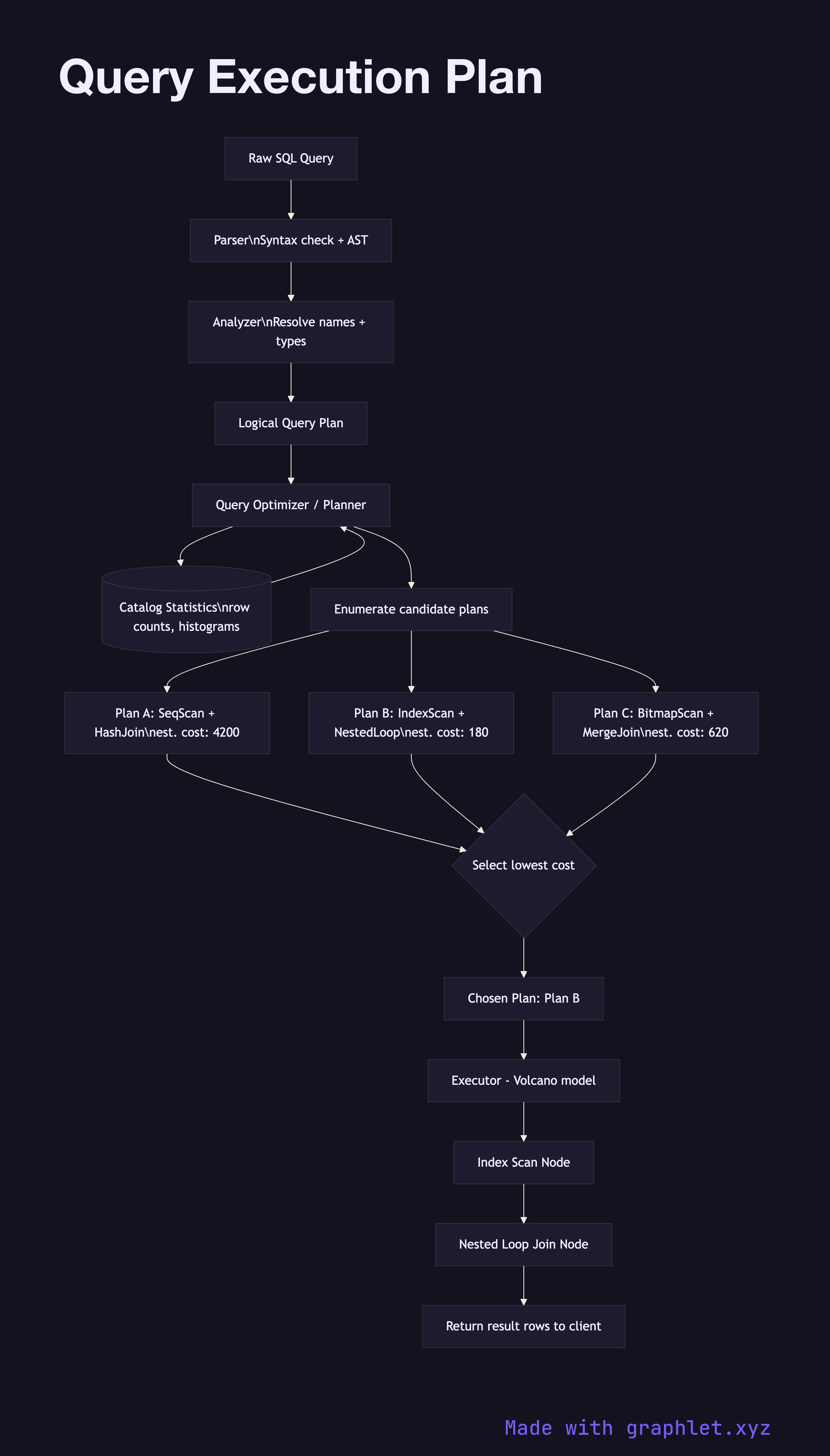
This diagram traces the pipeline from raw SQL to executed results. The query first passes through the parser, which checks syntax and produces an abstract syntax tree (AST). The analyzer then resolves table and column names against the catalog (system metadata), validates types, and expands wildcards. These two steps are purely structural and deterministic.

The resulting logical plan is handed to the optimizer (or planner). The optimizer enumerates possible execution strategies: for a table access, it considers sequential scan, index scan, bitmap index scan, and index-only scan. For joins, it considers nested loop, hash join, and merge join. Each strategy is assigned an estimated cost in arbitrary units based on statistics stored in the catalog (row counts, value distribution histograms, page counts). The optimizer picks the plan with the lowest estimated total cost.

The chosen plan is a tree of operator nodes — each node is an iterator that pulls rows from its children. For example, a hash join node pulls all rows from its inner child to build a hash table, then streams rows from its outer child to probe it. This iterator model is called the Volcano model and is used by PostgreSQL, SQL Server, and most traditional RDBMS engines.

When a plan is slow, the first diagnostic step is EXPLAIN ANALYZE (PostgreSQL) or EXPLAIN FORMAT=JSON (MySQL), which shows the actual plan, estimated vs. actual row counts, and execution time per node. Large discrepancies between estimated and actual rows indicate stale statistics — running ANALYZE (PostgreSQL) or OPTIMIZE TABLE (MySQL) refreshes them. The Database Index Lookup diagram explains how the planner chooses between scan strategies.

Frequently asked questions

A query execution plan is the ordered set of operations a database engine will perform to satisfy a SQL query. The query planner generates the plan by evaluating multiple possible strategies — different scan types, join algorithms, and operation orderings — and selecting the one with the lowest estimated cost based on table statistics.

The optimizer (or planner) receives a logical representation of the query and enumerates candidate physical strategies for each operation: sequential scan, index scan, or bitmap index scan for table access; nested loop, hash join, or merge join for joins. It assigns a cost to each strategy using catalog statistics (row counts, value distribution histograms) and selects the plan with the minimum estimated total cost.

Use `EXPLAIN ANALYZE` whenever a query is slower than expected or causes unexpected load on the database. It shows the actual execution plan alongside estimated vs. actual row counts and per-node execution time. Large row-count discrepancies (estimated 10 rows, actual 100,000) indicate stale statistics and a bad plan choice. Run `ANALYZE` to refresh statistics, then re-examine the plan.

The most common issue is an unwanted sequential scan on a large table due to a missing index or stale statistics. Fix by creating an appropriate index or running ANALYZE. Nested loop joins on large tables are another common bottleneck — the planner may choose them when it underestimates row counts, and increasing `work_mem` (PostgreSQL) can encourage a hash join instead. Occasionally, a query plan issue is caused by a parameter sniffing problem where a cached plan optimized for one parameter value performs poorly for another.

mermaid

flowchart TD
    SQL[Raw SQL Query] --> Parser[Parser\nSyntax check + AST]
    Parser --> Analyzer[Analyzer\nResolve names + types]
    Analyzer --> LogicalPlan[Logical Query Plan]

    LogicalPlan --> Optimizer[Query Optimizer / Planner]
    Optimizer --> Stats[(Catalog Statistics\nrow counts, histograms)]
    Stats --> Optimizer

    Optimizer --> CandidatePlans[Enumerate candidate plans]
    CandidatePlans --> Plan1[Plan A: SeqScan + HashJoin\nest. cost: 4200]
    CandidatePlans --> Plan2[Plan B: IndexScan + NestedLoop\nest. cost: 180]
    CandidatePlans --> Plan3[Plan C: BitmapScan + MergeJoin\nest. cost: 620]

    Plan1 --> CostCompare{Select lowest cost}
    Plan2 --> CostCompare
    Plan3 --> CostCompare

    CostCompare --> BestPlan[Chosen Plan: Plan B]
    BestPlan --> Executor[Executor - Volcano model]
    Executor --> ScanNode[Index Scan Node]
    ScanNode --> JoinNode[Nested Loop Join Node]
    JoinNode --> Results[Return result rows to client]