Partitioned Table Architecture: Mermaid Flowchart

Partitioned Table Architecture flowchart diagram

About Source

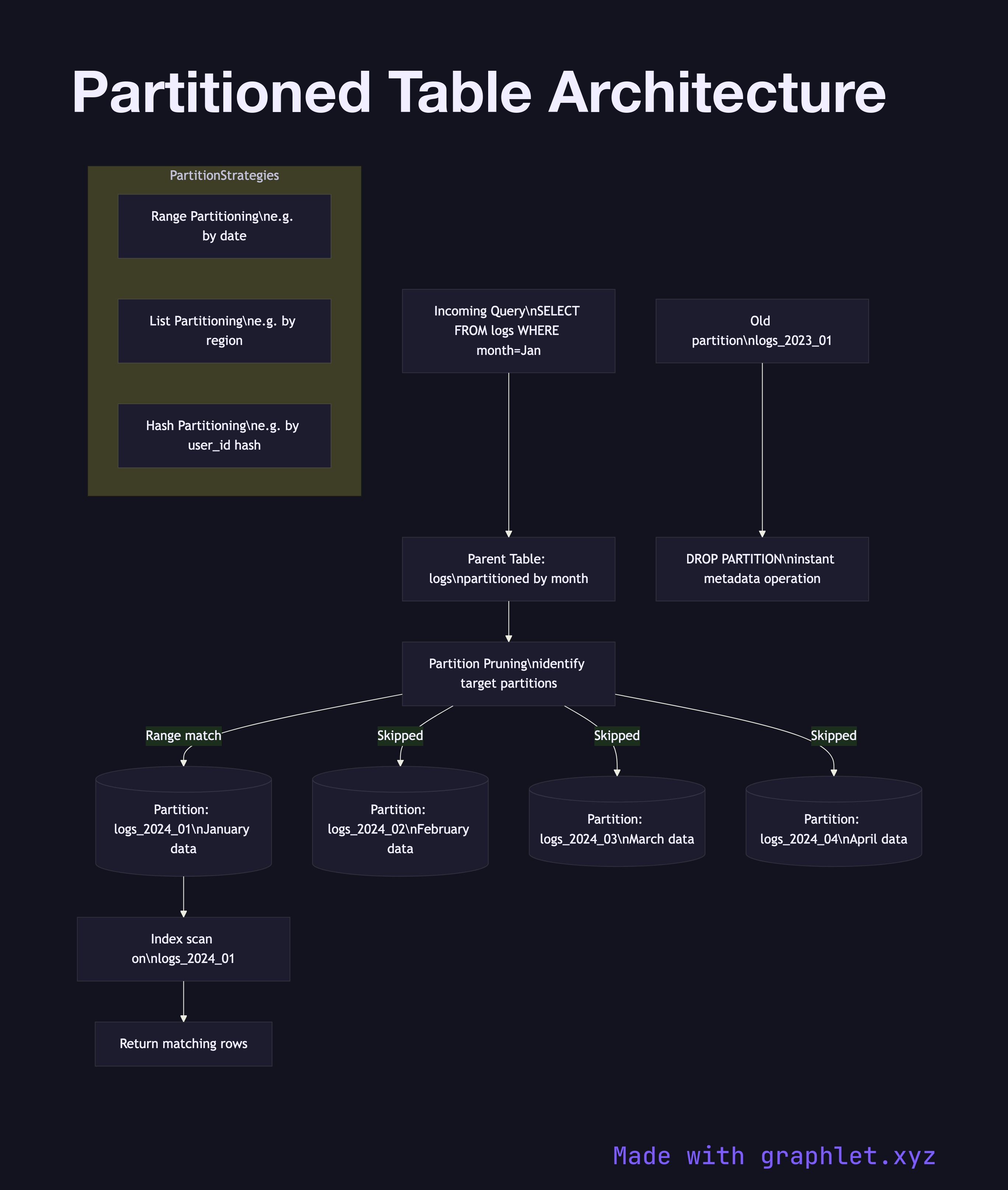
Table partitioning is a database technique that divides a large logical table into smaller physical sub-tables called partitions, each storing a subset of the rows, while the database engine presents them to queries as a single table.

This diagram shows how a partitioned table is structured and how queries route to the correct partitions. The parent table (also called the partitioned table) holds no data itself; it is a logical container that defines the partitioning key and strategy. Queries against the parent table are transparently routed by the partition pruning logic in the query planner.

There are three common partitioning strategies. Range partitioning assigns rows to partitions based on a value range — for example, a logs table partitioned by month, so January data lives in logs_2024_01, February in logs_2024_02, and so on. This is the most common strategy for time-series data. List partitioning assigns rows based on an explicit list of values — for example, a orders table partitioned by region with one partition per geographic region. Hash partitioning distributes rows evenly by hashing the partition key, similar in concept to Database Sharding but within a single database instance.

Partition pruning is the key performance benefit: a query with WHERE created_at BETWEEN '2024-01-01' AND '2024-01-31' only scans the January partition, skipping all others. Each partition can have its own indexes, tablespace, and even different storage parameters. Old partitions can be dropped instantly (a single metadata operation) rather than with slow DELETE statements.

The main operational cost is that queries without a partition key in the WHERE clause must scan every partition — a full partition scan that can be worse than a single unpartitioned table scan. Designing the partitioning key around your most common query predicates is critical.

Frequently asked questions

Table partitioning divides a large logical table into smaller physical sub-tables called partitions, each holding a subset of the rows. The database engine presents partitions as a single table to queries, while internally routing reads and writes to the correct partition based on the partition key.

Partition pruning is the planner's ability to exclude partitions that cannot contain rows matching the query's WHERE clause. A query with `WHERE created_at BETWEEN '2024-01-01' AND '2024-01-31'` on a month-partitioned table only scans the January partition, skipping every other partition entirely. This reduces I/O dramatically for time-series and range-filtered queries.

Use partitioning when your data volume challenges a single-instance database's query performance or manageability, but your write throughput is still within a single server's capacity. Partitioning works within one database instance and requires no application-layer routing. Use sharding when write throughput or total storage exceeds what a single instance can handle, requiring distribution across multiple independent servers.

mermaid

flowchart TD
    Query[Incoming Query\nSELECT FROM logs WHERE month=Jan] --> ParentTable[Parent Table: logs\npartitioned by month]
    ParentTable --> Pruning[Partition Pruning\nidentify target partitions]

    Pruning -->|Range match| P1[(Partition: logs_2024_01\nJanuary data)]
    Pruning -->|Skipped| P2[(Partition: logs_2024_02\nFebruary data)]
    Pruning -->|Skipped| P3[(Partition: logs_2024_03\nMarch data)]
    Pruning -->|Skipped| P4[(Partition: logs_2024_04\nApril data)]

    P1 --> IndexScan[Index scan on\nlogs_2024_01]
    IndexScan --> Result[Return matching rows]

    subgraph PartitionStrategies
        Range[Range Partitioning\ne.g. by date]
        List[List Partitioning\ne.g. by region]
        Hash[Hash Partitioning\ne.g. by user_id hash]
    end

    OldPartition[Old partition\nlogs_2023_01] --> DropPartition[DROP PARTITION\ninstant metadata operation]